

A Complete Wall Design
An out-of-plane wall design is complete when assemblage configuration design step, moment and deflection design step, and shear design step have been performed. Upon the completion of the out-of-plane wall design (whether it be successful or not), users have access to several output tabs. MASS is exceptionally transparent, providing the opportunity to quickly see exactly what equations the program used to achieve the design. This is extremely beneficial not only to users but to other designers that may review users’ work. As part of the results, the program provides detailed drawings that reflect the completed design, including: wall, loads, reactions, moment, shear, and deflection drawings, as well as a P-M diagram. The program also provides tabulated results. There are three result categories available for each module: simplified results, detailed results, and loads analysis results. The three result categories vary in the amount of detail provided, but all contain separate tables that approximately correspond to each design step. All drawings and results can be readily printed.
All results explored in this section assume a completed out-of-plane wall design. The drawings and tabulated results are often available in advance of a completed solution. The availability of a specific drawing or tabulated result is mentioned at each step during the design procedure.
Drawings
There are several useful drawings that the program provides in the out-of-plane wall module, including: Wall, Loads, Reactions, Moment, Shear, Deflection, and P-M Diagram
The first drawing becomes available as soon as the assemblage configuration design step is performed. The loads, reaction, moment, and shear drawings are not available until the loads input design step is performed.The deflection drawing and the P-M diagram are not available until the moment and deflection design step is performed. The out-of-plane drawing is updated at each design step to reflect any changes made to the assemblage. The drawings are not complete until all the design steps have been performed.
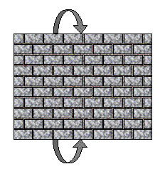
Wall
The wall drawing displays a wall with the material properties selected by users. The drawing displays the dimensions of the wall, as well as the detailed layout of the masonry units used in the design.The drawing also displays the reinforcement used in the wall.
To view the wall drawing, click on the Wall tab in the right window
For the wall module, all drawings are displayed in the right window, with the dimensions (height, length, width) of the out-of-plane wall clearly labelled, as shown in Figure 4‑36: Wall Drawing‑. The out-of-plane drawing includes the front (longitudinal) view, a side view, as well as a top (or cross-sectional) view of the wall.
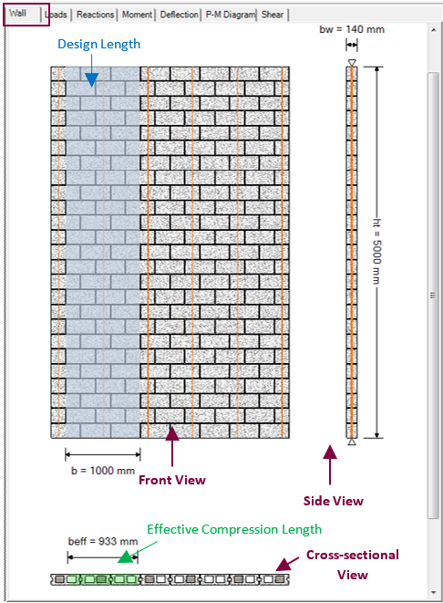
In the front (longitudinal) view, the program always displays a 3200 mm long wall.
The wall section selected in blue is the wall design length b . Since walls are typically designed per metre length, this design length is a fixed value of 1000 mm. The longitudinal view also shows the reinforcing bars (if applicable). Reinforcing bars normally extend out of the wall into the story above or other adjacent elements, in the program the bars are modelled as extending exactly to the end of the wall, no bends or hooks area shown.
![]() Warning: In the out-of-plane wall drawing, the vertical steel extends up to the ends of the wall as not to deceive users into thinking that the development length calculations had been performed. MASS does not perform any detailing work.
Warning: In the out-of-plane wall drawing, the vertical steel extends up to the ends of the wall as not to deceive users into thinking that the development length calculations had been performed. MASS does not perform any detailing work.
In the side view, the width (140 mm in Figure 4‑36: Wall Drawing) and height (5000 mm in Figure 4‑36: Wall Drawing) are displayed. This view also shows the reinforcing bars (if applicable).
In the cross-sectional view, the width, and length of the wall are shown (Figure 4‑36: Wall Drawing). The exact placement of the vertical steel is also shown (if applicable). In addition, the cross-sectional view provides the value for effective compression length, beff, selected in green (Figure 4‑36: Wall Drawing).
Loads
The loads drawing displays the loads that are applied to the wall. It is completed during the loads input design. To view the loads drawing:
- Click on the Loads tab (Figure 4‑37: Loads Drawing).
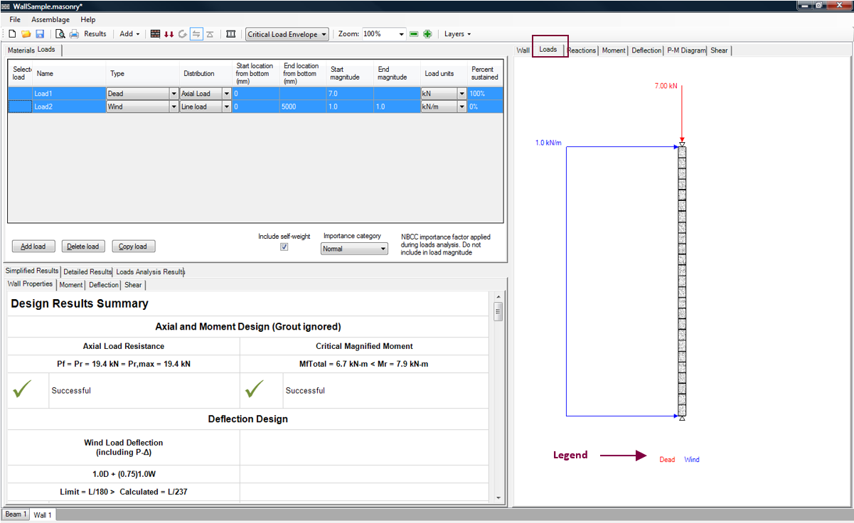
A specific applied load can be viewed under the Loads tab by clicking on the box of that particular load (under the ‘Selected load’ column). Multiple loads can be viewed by holding down Shift key, and selecting the loads to be displayed. Figure 4‑37: Loads Drawing shows two selected applied loads that are displayed in the loads drawing. The applied loads that are selected are highlighted in blue.
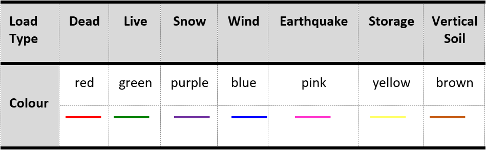
Each load type applied is displayed using a different colour (the legend is shown is displayed below the wall in the wall drawing). The dead load is displayed in red, and the live load is displayed in green. A full list of all load types available in the out-of-plane module, as well as their corresponding colour, are listed in Table 4‑4: Load Type Colour Convention‑.
Table 4‑4: Load Type Colour Convention
 Reactions
The reactions drawing displays the support reactions that are applied to the out-of-plane, due to a chosen load combination. It is initially displayed during the loads input design step. The drawing is updated at each design step to reflect any changes made to the assemblage. A change in the masonry unit size for instance, affects the self-weight of the wall, and thus the resulting support reactions.
To view the reactions drawing:
- Click on the Reactions tab Figure 4‑38: Reactions Drawing‑.
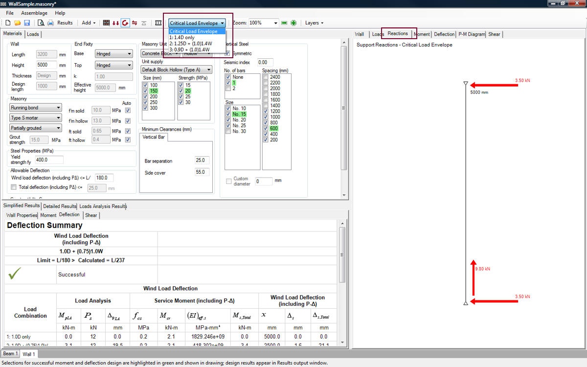 Figure 4‑38: Reactions Drawing
By default, the reactions drawing displayed uses the critical load envelope (formed by the worst case of all load combinations at any point in the wall). Reactions due to specific load combinations can be viewed by clicking on the Critical Load Envelope drop-down box, as shown in Figure 4‑38: Reactions Drawing‑. The drawing indicates at the top left corner the load combination used to determine that specific reaction.
Reaction forces (as well as moment and shear curves) are displayed using red, green, or both. Red is used to identify a positive reaction force (right to left). Green is used to identify a negative reaction force (left to right).
Moment reaction arrows follow a similar scheme. A red moment arrow at the top end of the wall indicates a positive moment reaction (counter-clockwise). A green arrow at the top end of the wall indicates a negative moment reaction (clockwise). A red arrow at the base of the wall indicates a positive moment reaction (clockwise). A green arrow at the base of the wall indicates a negative moment reaction (counter-clockwise).
![]() Note: The reaction drawing includes the reaction at the supports due to the self-weight of the wall.
Note: The reaction drawing includes the reaction at the supports due to the self-weight of the wall.
Moment
The moment drawing exhibits the bending moment along the height of the out-of-plane wall due to the applied loads and moments of a chosen load combination. It is completed during the loads input design step. The drawing is updated at each design step to reflect any changes made to the wall. A change in the masonry unit size for instance, affects the self-weight of the wall, the resulting support reactions, and thus the applied moment.
To view the moment drawing:
The bending moment diagram for a typical case of uniform positive bending, for a hinged-hinged supported wall, is shown in Figure 4‑39: Moment diagram. As a default, the program shows the factored moment for the ‘Critical Load Envelope’; however, other load cases (i.e.: 1.25D + 1.5L) can be displayed using the Critical Load Envelope drop-down menu. For the ‘Critical Load Envelope’ selection only, moment diagrams are displayed using red, green, or both. A red moment curve identifies a positive moment (in tension). |
Figure 4‑39: Moment diagram |
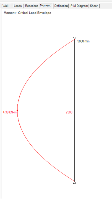
A green moment curve identifies a negative moment (in compression). Maximum absolute positive and negative moments are indicated as dots, (unless the maximum absolute moment is zero, i.e. there is no negative moment.) For all other load combinations the moment diagrams are displayed using a red curve.
Shear
The shear drawing displays the shear along the height of the wall due to the applied loads and moments of a chosen load combination. It is first displayed during the loads input design step. The drawing is updated at each design step to reflect any changes made to the out-of-plane wall.
To view the shear drawing:
- Click on the Shear tab in the right window
A shear diagram for a hinged-hinged supported wall is shown in Figure 4‑40: Actual Shear, Design Shear and Shear Resistance ‑.
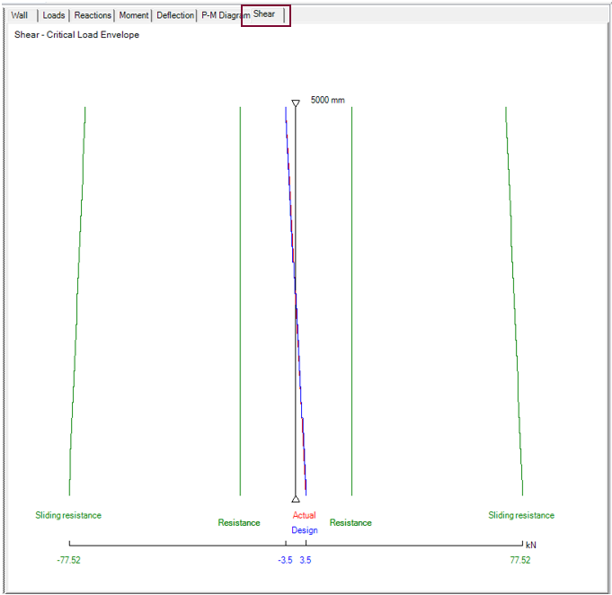
Figure 4‑40: Actual Shear, Design Shear and Shear Resistance
Completing the shear design step updates the shear drawing. In addition the actual (applied) shear (displayed at the loads input design stage), the shear resistance, and the sliding shear resistance at each masonry course are also displayed, as shown in Figure 4‑40: Actual Shear, Design Shear and Shear Resistance .
The actual shear is the shear the wall experiences due to the applied loads and moments. This curve is determined by the loads analysis engine and is plotted in red. The design shear is the factored shear the out-of-plane wall experiences, assuming the shear is constant along the height of each course of the wall (following CSA S304-14: 10.10.3). The shear resistance must exceed the design shear for the out-of-plane wall design to pass. This curve is drawn in blue in Figure 4‑40: Actual Shear, Design Shear and Shear Resistance . The shear resistance is the out-of-plane wall’s resistance to diagonal cracking, calculated in accordance to CSA S304-14: 10.10.3 for reinforced walls and CSA S304-14: 7.10.3 for unreinforced walls. This curve is drawn in green, and extends from first to last design cell. The sliding shear resistance is the out-of-plane wall’s resistance to out-of-plane sliding between bed joints, calculated in accordance to CSA S304-14: 7.10.5.2 and CSA S304-14: 10.10.5.2.
The shear diagram corresponding to a specific load combination can be viewed by clicking on the Critical Load Envelope drop-down box. The drawing indicates at the top left corner the load combination used to determine that specific shear diagram. A shear drawing with the design shear is available only for the critical load combination since this is the load combination the design shear is determined for. The actual shear and shear resistance can be viewed for all load combinations.
![]() Note: The critical load combination for the step shear design may be different than the critical load combination for the moment and deflection design step.
Note: The critical load combination for the step shear design may be different than the critical load combination for the moment and deflection design step.
Deflection
The deflection drawing displays the deflection of the out-of-plane wall due to the applied loads and moments of a chosen load combination. It is first displayed during the moment and deflection design step. The drawing is updated at each design step to reflect any changes made to the assemblage. To view the deflection drawing:
- Click on the Deflection tab in the right window (Figure 4‑41: Deflection Drawing).
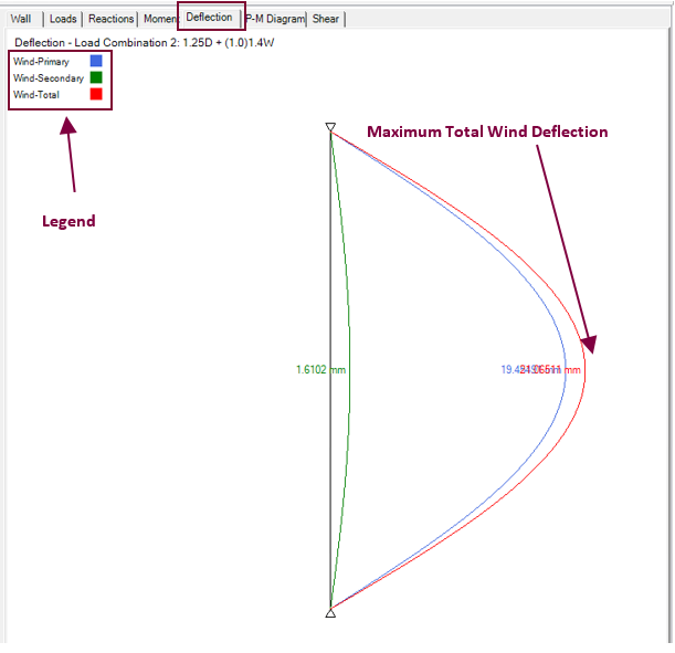
Figure 4‑41: Deflection Drawing
Notice that in Figure 4‑41: Deflection Drawing the deflection drawing is displayed for the Load Combination 2: 1.25D+(1.0)1.4W in this example. A specific load combination can be selected using the Critical Load Envelope drop-down box.
For this load combination, primary wind load deflection, secondary wind load deflection, and total wind load deflection the wall experiences are displayed using different colours (the legend is featured in the top left corner of the beam drawing). Description of these deflections, as well as other common deflection terms are provided in Table 4‑5: Deflections Displayed in Deflection Drawing‑.
Table 4‑5: Deflections Displayed in Deflection Drawing
|
Deflection |
Description |
| Wind (Primary) | Primary deflection as a result of lateral (horizontal) wind loads. This includes point loads, line loads, and applied moments of the wind type. |
| Wind (Secondary) | Secondary deflection as a result of the primary deflection. Calculated using the P-Δ method. Axial load types which can contribute to secondary deflection are; dead, live, snow, wind, hydrostatic, storage, controlled fluid, and soil (all available loads except for earthquake). |
| Wind (Total) | Wind deflection determined by adding the primary wind deflection and secondary wind deflection. |
| Total (Primary) | Primary deflection as a result of all lateral (horizontal) loads. This includes point loads, line loads, and applied moments of the any applied type. |
| Total (Secondary) | Secondary deflection as a result of the primary deflection. Calculated using the P-Δ method. Axial load types which can contribute to secondary deflection are; dead, live, snow, wind, hydrostatic, storage, controlled fluid, and soil (all available loads except for earthquake). |
| Total | Total deflection determined by adding the primary total deflection and secondary total deflection. |
P-M Interaction Diagram
After achieving a successful axial, moment and deflection design, the program creates an axial resistance, Pr , vs. moment resistance, Mr , diagram. The P-M interaction diagram also displays the axial force Pf and the principal moment, Mfp, and the total (magnified) moment, Mf,total , and for every load combination, the program displays. A thin horizontal black line connects the two points, providing users with a clear picture of the slenderness magnification effect.
The calculation procedure and the curves displayed in the P-M interaction diagram depend on whether the wall is reinforced or not, and whether the masonry is hollow, partially grouted or fully grouted.
For unreinforced walls, moment resistance, Mr, is determined and plotted for incremented values of the axial resistance, Pr . The moment resistance calculations vary depending on whether the wall is designed as an uncracked or a cracked section. A full discussion on the possible P-M Diagram configurations for unreinforced walls is provided in the P-M Interaction Diagram section.
To view the P-M diagram:
- Click on the P-M Diagram tab in the right window
A sample P-M Interaction diagram for a hinged-hinged supported unreinforced, fully grouted wall is shown in Figure 4‑42: P-M Interaction Diagram for an Unreinforced, Fully Grouted Wall‑.
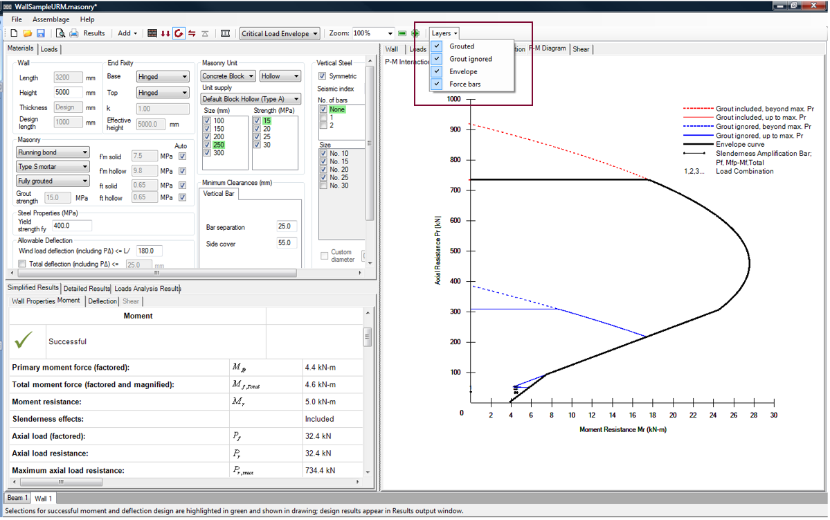
Figure 4‑42: P-M Interaction Diagram for an Unreinforced, Fully Grouted Wall
For drawings available in MASS, users are permitted to select the amount of detail displayed in each drawing. This feature becomes especially useful for P-M diagrams. With the Layers drop-down box, users can choose to include or exclude several P-M diagram features. For an unreinforced, fully grouted wall for instance, the following layers can be included or excluded:
- Resistance curve when grout is ignored
- Resistance curve when grout is included
- Resistance envelope curve
- Slenderness amplification bars (sometimes referred to as ‘Walls: Force bars’)
For a grouted wall (Figure 4‑42: P-M Interaction Diagram for an Unreinforced, Fully Grouted Wall), the design approach used within MASS unique: the program provides separate curves depending on whether or not the effect of the grout is included.
For the ‘Grout ignored’ curve, the compression strength of hollow masonry (fm, hollow ) is used, independent of the depth of the compression zone. In Figure 4‑42: P-M Interaction Diagram for an Unreinforced, Fully Grouted Wall the solid blue line represents the Pr,Mr values ignoring the effects of grout, up to the maximum axial load allowed Pr,max .r,Mr values ignoring the effects of grout, when the axial resistance has exceeded the maximum axial load.
For the ‘Grouted’ curve, the compressive strength of the masonry depends on the depth of the compression zone. If the depth of the compression zone falls in the face shell, f’m,hollow is used (calculated using CSA S304-14: Table 4). If the depth of the compression zone is greater than the width of the face shell, and the wall is fully grouted, f’m,grouted is used (calculated using CSA S304-14: Table 4). In Figure 4‑42: P-M Interaction Diagram for an Unreinforced, Fully Grouted Wall the solid red line represents the Pr,Mr values including the effects of grout, up to the maximum axial load allowed, Pr,max . The dotted red line represents the Pr,Mr values including the effects of grout when the axial resistance has exceeded the maximum axial load.
Notice that when using CSA S304-14: Table 4, the grouted compressive strength, f’m,grouted , is smaller than the hollow compressive strength,f’m,hollow . Thus, when the compression zone is just outside the first face shell it is possible for moment resistance of the wall to be smaller when the grout is included than when it is not. In practice, adding grout does not reduce the moment capacity of the wall, hence, it is permissible to ignore the effect of grout if it is advantageous. To ensure that the addition of grout does not reduce the capacity of a wall, a comparison between the moment resistances yielded when excluding the grout and including the grout is performed. The largest resulting moment resistance is used by the program to determine a successful design. This is illustrated with the help of the envelope curve. The envelope curve (black line) indicates the moment resistance and axial resistance values used to achieve the design.
To determine an exact data point on the envelope, place the mouse cursor on the black curve and left-click, as shown in Figure 4‑43: P-M Interaction Diagram (Envelope Data Points)‑.
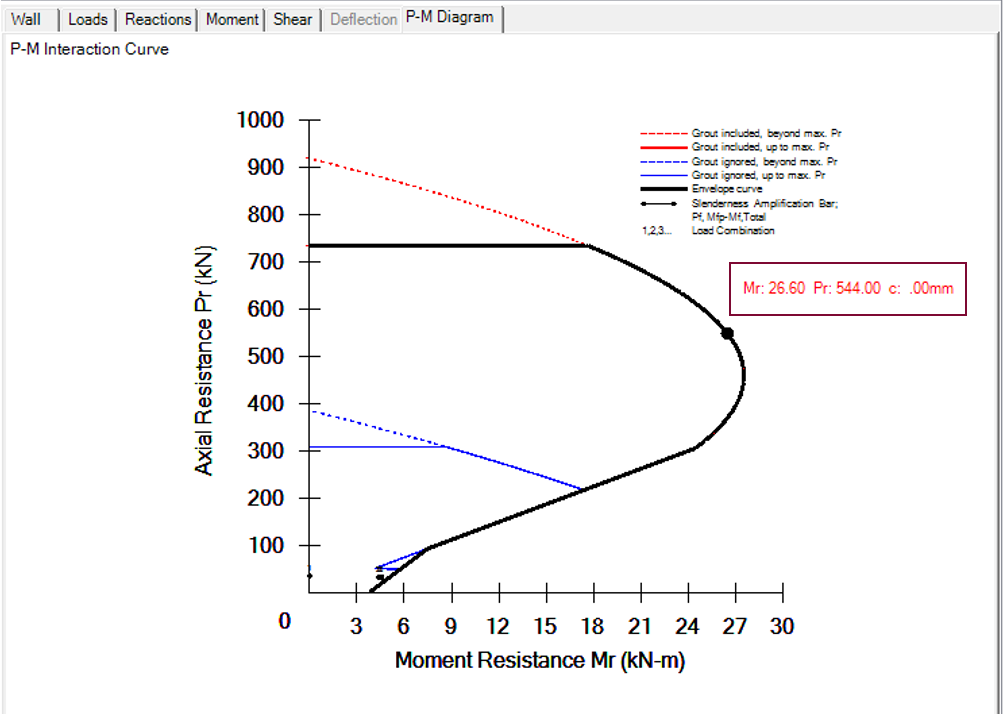
Figure 4‑43: P-M Interaction Diagram (Envelope Data Points)
The moment resistance, axial resistance, and neutral axis used in the design are displayed in red, next to the selected point. Notice that in Figure 4‑43: P-M Interaction Diagram (Envelope Data Points)‑ the neutral axis value is zero. This is because this particular wall is designed to remain uncracked (following CSA S304-14: 7.2.3). For uncracked walls, the moment resistance is calculated (following CSA S304-14: 7.2.4) for increasing increments of the axial resistance, and no neutral axis value is determined.
In addition to the resistance curves drawn in the P-M Interaction diagram, the program also displays the axial force and the principal moment Pf, Mfp and the axial force and the total (magnified) moment Pf, Mf, total for every load combination. The slenderness amplification bar, a thin horizontal black line connects the two points, providing users with a clear picture of the magnification effect. Each slenderness amplification bar is labelled with a number, indicating the corresponding load combination. For a design to be successful, all slenderness amplification bars must lie within the envelope curve.
The P-M interaction diagram for the out-of-plane wall design shown in Figure 4‑44: Slenderness Amplification Bars is just one example. There are many other possible P-M diagram configurations. The shape of the P-M diagram depends on the specific design. For reinforced walls for example, the axial resistance, Pr, and the moment resistance, Mr, are determined and plotted for incremented values of the neutral axis depth c. The neutral axis depth begins with c=1 mm and is incremented up by 1 mm with each iteration, terminating when the compression zone is equal to the thickness of the block (when β1c=1).
A sample P-M Interaction diagram for a hinged-hinged supported reinforced, partially grouted wall is shown in Figure 4‑44: Slenderness Amplification Bars.
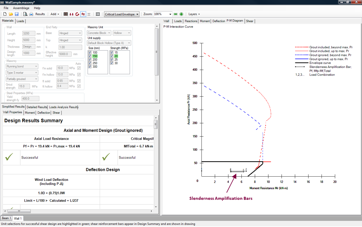
Figure 4‑44: Slenderness Amplification Bars
MASS does not account for reinforcement in compression in the moment resistance calculations, since tying bars in walls is not easily accomplished. Consequently, in the case where neutral axis depth is equal to the depth of the main (tension) reinforcement layer c=d1, where the steel transitions from being in tension to being in compression, the moment resistance varies considerably upon the smallest increment of c. This results in missing moment resistance and axial resistance data points in between this transition zone (discussed in greater detail in the following section).
Transition Zone
For out-of-plane reinforced walls, the P-M diagram is drawn by varying the length of the neutral axis c and determining the corresponding axial resistance and moment resistance of the wall. For reinforced walls, when the neutral axis depth extends the location of the steel, the steel is no longer in tension, and the wall can be treated as unreinforced. The resistance of the wall may change considerably because the compression zone length (beff ) varies depending on if the wall is treated as reinforced (when the reinforcing steel is in tension), or if the wall is treated as unreinforced (when the reinforcing steel is in compression). This jump from being reinforced to unreinforced may produce a considerable discontinuity in the P-M diagram. Within the program, this discontinuity is deemed the transition zone. For MASS, the point at which the steel is still in tension is deemed Mr,tension,Pr,tension, the point at which the steel is in compression is deemed Mr,compression,Pr,compression. Theoretically, these two points share the same neutral axis value c, but are calculated using the appropriate beff .
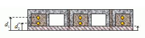
For example, for a 1.2 m wall designed using 20 cm unit blocks, with bar spacing at 1.2 m, when the bar is in tension, the compression zone length is calculated using CSA S304-14: 10.6.1 (assuming running bond pattern), as follows:

This compression zone length is illustrated in Figure 4‑45: Compression zone length , when .
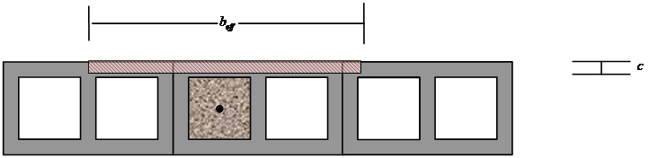
Figure 4‑45: Compression zone length beff , when c<d1
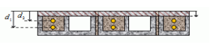
For a 1.2 m wall with bar spacing at 1.2 m, when the bar is in compression, the compression zone length is 1000 mm (the entire design length of the wall), as shown in Figure 4‑46: Compression zone length when ‑.
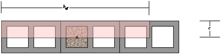
Figure 4‑46: Compression zone length beff when c<d1
The change in the compression zone length, beff results in a jump in the axial resistance and moment resistance data points. In order to create a smoother transition in the P-M diagram, while maintaining a conservative design, the program takes special design considerations depending on the circumstance in which the transition zone is encountered. For larger reinforcement spacings, the transition zone becomes more prominent, because of how the compression zone length is calculated:

For spacings smaller or equal to four times the actual thickness the compression zone length remains at 1000 mm, and therefore there is no noticeable transition zone.
A full discussion on the possible P-M Diagram configurations for reinforced walls is provided in the P-M Interaction Diagram section.
Simplified Results
There are three tabulated result categories available in the out-of-plane wall module: simplified results, detailed results, and loads analysis results. The three result categories vary in the amount of detail provided, but all contain separate tables that approximately correspond to each design step, as shown in Figure 4‑47: Tabulated Results Categories for Out-of-Plane Module: Simplified, Detailed, Loads Analysis‑.
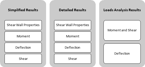
Figure 4‑47: Tabulated Results Categories for Out-of-Plane Module: Simplified, Detailed, Loads Analysis
The simplified results show only those values that are required to give an overview of the results for a design criterion. The simplified results tab contains four tabs which provide design summaries for including:
- Wall Properties
- Moment
- Deflection
- Shear
The first three of tabs become available as soon as the moment and deflection design step is performed. The Shear tab is not available until the shear design step is performed. The Simplified Results tabs are updated at each design step to reflect any changes made to the wall design. The four Simplified Results tabs are not complete until all the design steps have been performed.
Wall Properties
The Wall Properties tab is activated after the moment and deflection design are performed. To view the simplified results, wall properties:
- Click on the Simplified Results tab
- Click on the Wall Properties tab
The Wall Properties tab contains a summary table (titled ‘Design Results Summary’) that quickly advises users of the design stages that have been satisfied. Design steps that have been satisfied, and provided a successful design, are indicated with a green check mark. The design steps that have been satisfied, but did not provide a successful design, are indicated with a red ‘X’. Design steps that are yet to be performed are indicated with a blue horizontal line, as can be seen in Figure 4‑48: Simplified Results (Wall Properties, Design Step Status).
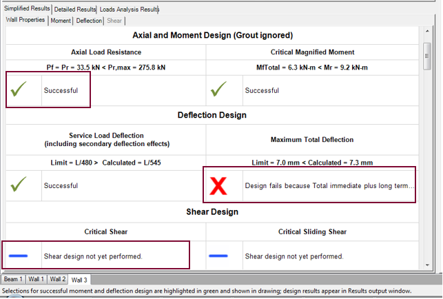
Figure 4‑48: Simplified Results (Wall Properties, Design Step Status)
The out-of-plane wall designed in the Wall Design Steps section with all design steps completed in shown in Figure 4‑49: Simplified Results (Wall Properties)‑.
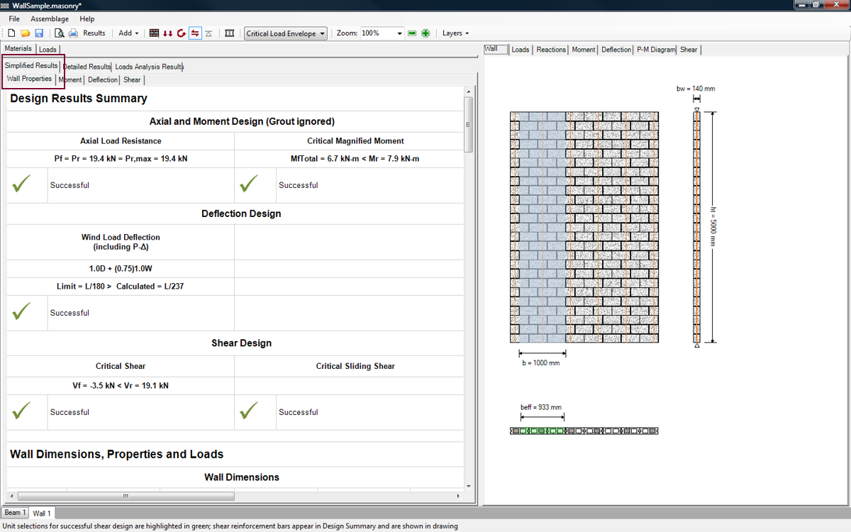
Figure 4‑49: Simplified Results (Wall Properties)
At the top of the ‘Design Results Summary’ page, the moment and deflection design step is summarized. The program displays the factored magnified moment, Mf,Total, (for the critical load combination) and the moment resistance, Mr ,(for the critical load combination). While Mf,total is determined for every load combination, the critical load combination is the load combination that results in the smallest Mr/Mf,Total. This is the moment that the wall is designed for. This is discussed further under the ‘Slenderness Effects’ section.
In addition to providing the critical magnified moment and the moment resistance, the ‘Design Results Summary’ indicates whether or not the moment resistance includes the effects of grout or not. In the design example shown in Figure 4‑49: Simplified Results (Wall Properties), the moment resistance, Mr, displayed corresponds to the moment resistance calculated by excluding the effects of grout. This means that for this particular design, the moment resistance determined by excluding the grout is larger than the moment resistance determined by including the grout.
The program also shows the factored axial load, Pf, the axial load resistance,Pr, and the maximum axial load resistance, Pr,max. The factored axial load is simply the factored applied axial load that corresponds to the critical load combination. For out-of-plane walls, the program sets the axial load resistance equal to the factored axial load, and solves for the neutral axis depth Pr,max. Thus the axial load resistance is always be equal the factored axial load.
For deflection design, the program displays the service wind load deflection (including slenderness effects), and the wind deflection limit. The program also displays the total load deflection, and the total deflection limit (if one is entered by the user).
For shear design, MASS shows the factored shear, Vf , the shear resistance, Vr, and the factored sliding shear at the critical section, as well as the critical sliding shear resistance. The critical section corresponds the location along the height of the wall that results in the smallest Vr/Vf ratio. Scrolling down further along the ‘Design Summary Results’ page, the wall properties and the applied load information are provided (Figure 4‑50: Simplified Results (Wall Properties)‑). The wall properties provided include the wall dimensions, support information, masonry properties, as well as the unit properties used to attain the wall design.
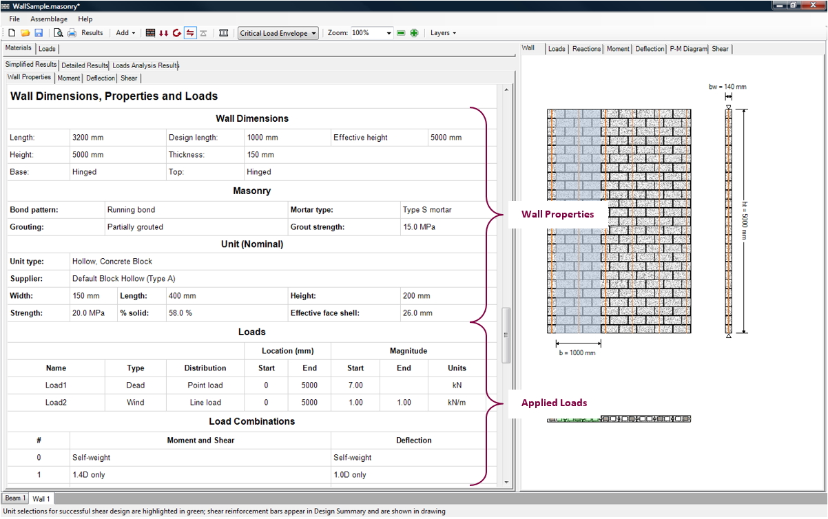
Figure 4‑50: Simplified Results (Wall Properties)
The applied loads information includes a list of all the loads applied to the wall (along with their location, and unfactored magnitude), a list of all the load combinations (used in the moment and deflection design step, and the shear design step), as well as a list of all the load types applied by the user.
Moment
The Moment tab is activated after the moment and deflection design step is performed. To view the simplified results, moment:
- Click on the Simplified Results tab
- Click on the Moment tab
The Moment tab contains a summary table (titled ‘Moment Design Summary’) that quickly advises users of the success or failure of the moment design. A green check mark is used to indicate a successful moment design, as shown in Figure 4‑51: Simplified Results (Moment tab). If the design is not successful, it is indicated with a red ‘X’.
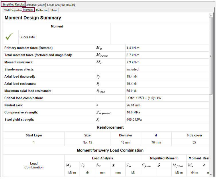
Figure 4‑51: Simplified Results (Moment tab)
At the top of the ‘Moment Design Summary’ page, program provides the factored primary moment, Mfp, the factored total (magnified) moment, Mf,total, and the moment resistance Mr , for the critical load combination. The factored primary moment is the bending moment due to the applied loads. The total moment is the magnified bending moment (includes the slenderness effects if applicable). The ‘Moment Design Summary’ page also informs users if slenderness effects are included, or if they can be neglected. In the design example shown in Figure 4‑51: Simplified Results (Moment tab) slenderness effects are included. In instances where slenderness effects are neglected, Mf,total=Mfp. For more information on slenderness effects, refer to the following section.
The ‘Moment Design Summary’ provides the factored axial load (for the critical load combination), Pf , the maximum axial load resistance,Pr , the critical load combination, and the neutral axis depth, c. It also provides the properties of the vertical reinforcement, number of bars per cell, bar size, bar location in the wall, and side cover of the vertical reinforcement.
Scrolling further down, the compressive strength displayed is the strength of the masonry, based on the resulting design. The yield strength of the steel is simply the value entered by users (usually during the assemblage configuration design step). This value by default is 400 MPa.
Slenderness Effects (Moment Magnifier)
The slenderness of the wall plays an important role in determining the resistance of the wall. If the wall slenderness ratio exceeds slenderness ratio limits specified in CSA S304-14: 7.7.5 and, 10.7.3, the moment magnifier method or P-Δ method must be applied to account for slenderness effects. In MASS, the moment magnifier method (described in CSA S304-14: 7.7.6.3, and 10.7.4.3) is used for moment calculations. The factored primary moment (Mfp) is magnified using a magnification factor to calculate a total factored moment (Mf,total) (determined for every load combination). The wall must be able to resist, Mf,total, for the critical load combination.
The moment magnifier method requires determining a magnification factor that is dependent upon the critical axial compressive load, Pcr, the, Cfactor(the factor that relates the actual moment diagram to the equivalent moment diagram and depends on the end moments), and, ßd(the ratio of the factored dead load moment to the factored total moment). The moment magnifier is also dependent upon the effective stiffness of the wall. The magnification factor determined is then used to multiply the moment for each load combination.
Note: There is an important distinction between applying slenderness effects to a wall, and a slender wall. A wall that experiences slenderness effects is not automatically a slender wall. Including slenderness effects implies the designer taking into account the fact that the bending moment a wall experiences can be affected by the slenderness of the wall. Slenderness effects must be applied to walls that are non-slender but have a slenderness ratio of:  as well as slender walls (walls that have a slenderness ratio greater than 30).
In the Simplified Results tab, the calculations performed to determine the slenderness effects are displayed towards the bottom of the ‘Moment Design Summary’ page. The primary moment, resulting total factored moment, and moment resistance are also displayed for every load combination, as shown in Figure 4‑52: Simplified Results (Magnified Moment for Every Load Combination)‑.
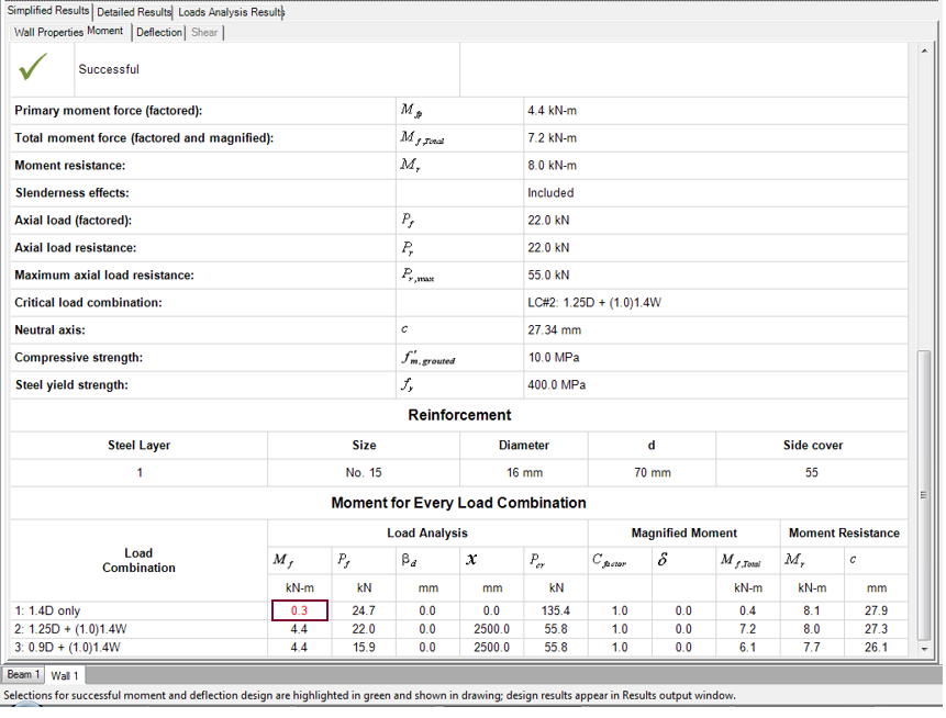
Figure 4‑52: Simplified Results (Magnified Moment for Every Load Combination)
Minimum Primary Moment
According to CSA S304-14: 10.7.2, if the factored moments due to the applied loads (lateral or axial) result in a primary bending moment that is less than Pf(0.1t) a minimum moment of Pf(0.1t) should be applied to the wall.
The program automatically applies this minimum moment for every load combination (where applicable). When a minimum primary moment is applied, it is distinguished using red font, as shown and highlighted in Figure 4‑52: Simplified Results (Magnified Moment for Every Load Combination)‑.
Deflection
To view the ‘Deflection Design Summary’:
- Click on the Simplified Results tab
- Click on the Deflection tab
The Deflection tab contains a summary table (titled ‘Deflection Design Summary’) that quickly advises users if the deflection design (during the moment and deflection design step) has been satisfied. The Deflection tab also contains a summary of the deflection calculations performed by the program (Figure 4‑53: Simplified Results (Deflection tab)‑).
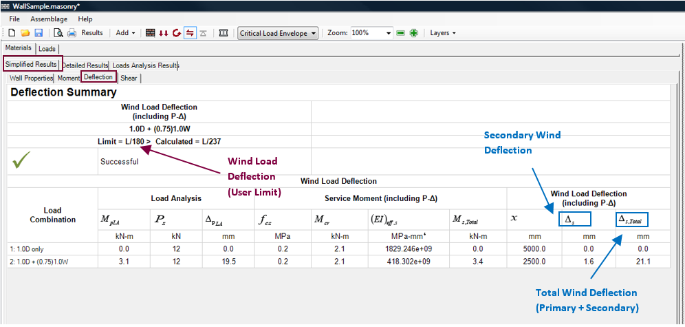
Figure 4‑53: Simplified Results (Deflection tab)
In cases where the user chooses to place a limit on the total deflection of the wall, an additional set of rows is provided by the program.
Slenderness Effects (P-Δ)
The Simplified Results → Deflection tab provides the summarize wind load deflection (including P-Δ effects) and the total deflection (including P-Δ effects), as well as the corresponding limits and the corresponding critical load combinations.
The slenderness of the wall plays an important role in determining the resistance of the wall. If the wall slenderness ratio exceeds slenderness ratio limits specified in CSA S304-14: 7.7.5 and, 10.7.3, the moment magnifier method or P-Δ method must be applied to account for slenderness effects. In MASS, the P-Δ (described in CSA S304-14: 7.7.6.2, and 10.7.4.2) is used to account for these effects when calculating the service load deflections. The primary wind load deflection, ∆pLA , and secondary wind load deflection, ∆s, are added to determine the total wind load deflection ∆s,Total . The primary total deflection ,∆pLA, and secondary total deflection, ∆s, are added to determine the total deflection, ∆s,Total. The deflections are determined for every load combination.
The Simplified Results → Deflection tab also displays the maximum primary and secondary wind and total deflections for each load combination. To determine these deflections, the program first determines: the unfactored moment, MpLA, unfactored axial force, Ps, and deflection, ∆pLA. These are retrieved from the loads analysis engine, determined using finite element analysis, prior to the inclusion of slenderness effects. The cracking moment, Mcr, moment of inertia, (EI)eff,s and the total service moment Ms,total (including slenderness effects) are then determined. For more information on the P-Δ method, refer to the Moment and Deflection Design Strategy section.
Note: For unreinforced masonry walls, no deflection calculation is completed. CSA S304 does not provide provisions for calculating the deflection of URM walls. This is because the out-of-plane wall cannot deflect without significant cracking. A URM that experiences significant cracking cannot pass moment design provisions outline in CSA S304.
For more information on the P-Δ method, refer to the Moment and Deflection Design Strategy section.
Shear
The Shear tab is activated after the shear design is performed. To view the simplified results for shear design:
- Click on the Simplified Results tab
- Click on the Shear tab
The Shear tab contains a summary table (titled ‘Shear Design Summary’) that quickly advises users of the success or failure of the shear design (critical shear, and critical sliding shear). If the shear design step is satisfied, it is indicated with a green check mark (see Figure 4‑54: Simplified Results (Shear)); if not, it is indicated with a red ‘X’.
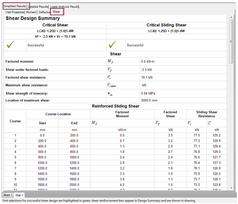
Figure 4‑54: Simplified Results (Shear)
At the top of the ‘Shear Design Summary’ page, the program provides the factored moment, Mf, at the location of maximum shear.
The program also displays the factored shear,Vf , and the critical out-of-plane shear resistance, Vr, at the critical section, for the critical load combination. For out-of-plane shear, the critical load combination is the one with the smallest shear resistance to factored shear ratio along the wall height,. The critical section corresponds to the location along the height of the wall that results in the smallest Vrd/Vf ratio.
![]() Note: The critical load combination may not be the same for moment design as it is for shear design.
Note: The critical load combination may not be the same for moment design as it is for shear design.
Notice in Figure 4‑54: Simplified Results (Shear) that Vr is significantly larger than Vf. For out-of-plane walls, the shear resistance of masonry walls is typically much higher than the factored applied loads. As in the beam module, axial compression loads enhance the shear resistance of walls. Because walls are vertical elements, the wall’s self-weight also helps resist shear. Walls are also more resistant to out-of-plane shear than beams because the tensile and compressive internal forces, act perpendicular to the bed joints, allowing the use of the total magnitude of the compressive strength of the masonry (in contrast to beams, where only 50 or 70 % of the compressive strength is allowed to be used).
The out-of-plane shear resistance is calculated in accordance to CSA S304-14: 10.10.2 for reinforced walls and CSA S304-14: 7.10.2 for unreinforced walls. It represents the resistance of the wall to diagonal cracking, as shown in Figure 4‑55: Diagonal Crack Due to Out-of-Plane Shear‑. In order to increase the out-of-plane shear resistance of the wall one must increase the strength of the masonry itself. Unlike with beams and shear walls, there is no additional shear reinforcement that can be included for out-of-plane shear behaviour.
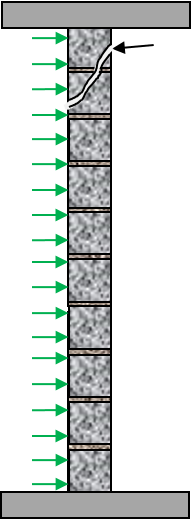
Figure 4‑55: Diagonal Crack Due to Out-of-Plane Shear
At the top of the ‘Shear Design Summary’ page, the program also provides the factored sliding shear, Vf, and the critical sliding shear resistance, Vr, at the critical section, for the critical load combination. For sliding shear, the critical load combination is the one with the smallest shear resistance to factored shear ratio (Vr,j/Vf,j). The critical section corresponds to the location along the height of the wall that results in the smallest Vr,j/Vf,jratio.
Notice in Figure 4‑54: Simplified Results (Shear) that Vr is significantly larger than Vf. For out-of-plane walls, the sliding shear resistance of masonry walls is typically much higher than the factored applied loads at each course. As shown in Figure 4‑56: Sliding Due to Out-of-Plane Shear‑, lateral loads, like wind pressure, can produce sliding shear failure between the bed joints of the masonry wall (horizontal plane). The sliding shear resistance between bed joints is calculated using CSA S304-14: 7.10.5.2 (unreinforced wall) or 10.10.5.2 (reinforced wall).
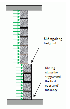
Figure 4‑56: Sliding Due to Out-of-Plane Shear
Scrolling down further along the ‘Shear Design Summary’ page, the program provides the factored sliding shear, sliding shear resistance, and compression force at each course. Notice that the sliding shear resistance is determined at each course. The program does not calculate the sliding shear at the base of the wall. It is the responsibility of users to verify the sliding shear resistance at the base of the wall, taking into account the friction coefficient of materials in contact (masonry-to-smooth concrete or bare steel), and dowels (if any).
For information about the shear design strategy, refer to the Shear Design Strategy section.
Detailed Results
The detailed results provide the intermediate calculations performed to obtain the final wall design. The detailed results are organized into tables that include:
- Variables used in the design
- Calculated result (of the successful design run, or the last unsuccessful design run)
- Units employed
- Engineering equations (or descriptions of the origin of the values in the absence of equations)
- CSA standard reference (where applicable).
The detailed results contain four tabs which provide design information for:
- Wall Properties
- Moment
- Deflection
- Shear
The first three of tabs become available as soon as the moment and deflection design step is performed. The Shear tab is not available until the shear design step is performed. The Detailed Results tabs are updated at each design step to reflect any changes made to the wall design. The four Detailed Results tabs are not complete until all the design steps have been performed.
Wall Properties
To view a full list of the wall properties:
- Click on the Detailed Results tab
- Click on the Wall Properties tab
The Wall Properties tab contains a table that provides detailed information about the wall geometry, the reinforcement cover and spacing values, and any applicable constants and factors. In general, the data presented in this Wall Properties tab is common to more than one design step (Figure 4‑57: Detailed Results (Wall Properties)‑).
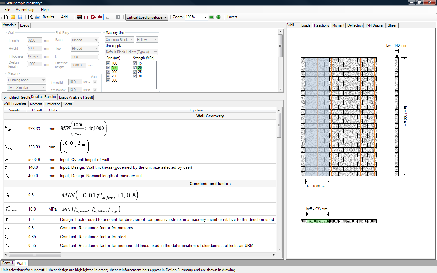
Figure 4‑57: Detailed Results (Wall Properties)
Most variables displayed in the Detailed Results → Wall Properties tab are variables commonly used and follow the convention presented in CSA S304-14. In cases where the variable/symbol is not governed by a specific equation, a description of the variable is provided instead. Variables and equations that may require further explanation are discussed in the following subsections.
Effective Compression Zone Length
The effective compression length beff, is the length of the wall that acts with a single reinforcing bar (for walls under minor axis bending), adjusted to a per meter length. It varies depending on if the wall is being reinforced or unreinforced, the reinforcement spacing, and the bond pattern (running bond, or stack bond). If the wall is unreinforced, or if it is reinforced but the bars are in compression, the effective compressive length is equal to 1000 mm. Otherwise, the length is reduced according to CSA S304-14: 10.6.1. To determine the effective face shell compression zone length, the program calculates the width of section acting with a single reinforcing bar, using![]() for running bond, and
for running bond, and  for stack bond.
In addition to the compression zone length, the program also determines the web compression zone length, bw,eff. For a partially grouted wall, the hollow and grouted areas can be treated separately, as illustrated in Figure 4‑58: Effective Compression Zone Length‑.
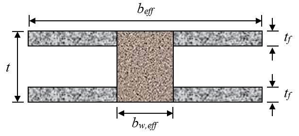
Figure 4‑58: Effective Compression Zone Length
In the case of the effective web compression zone design length, the program differentiates between hollow, partially, or fully grouted walls. If the wall is partially grouted, the length of compression zone over the grout is directly related to the spacing of reinforcement,  . If the wall is not grouted (hollow), the length of compression zone over the grout is ‘zero’, bw,eff=0. If the wall if fully grouted, the length of compression zone over the grout is equal to the effective face shell compression zone length, bw,eff=beff.
Notice that in the Detailed Results tab shown in Figure 4‑57: Detailed Results (Wall Properties), there may be two different beff values (a value for when grout is included and a value for when it is ignored). The final beff used in the design is displayed in wall drawing (Figure 4‑36: Wall Drawing).
Depth Ratio of Compression Block
Just like for concrete design, the rectangular stress block can be used in masonry design to simplify calculations of the resultant compression force at ultimate strength. The ratio of depth of rectangular compression stress block to depth to neutral axis, , helps define the rectangular compression block. ßl is 0.8 for masonry compressive strength values equal and less than 20 MPa. For compressive strength values greater than 20 MPa, ßl decreases at a rate of 0.1 for each increase of 10 MPa above 20 MPa compressive strength, following CSA S304-14: 10.2.6. For unreinforced walls, this factor is calculated using f’m,hollow for an ungrouted wall and f’m,grouted for a grouted wall. For reinforced walls, this factor is calculated using the minimum off’m,hollow,f’m,grouted, and f’m,eff to maintain a conservative design.
Stress Orientation Factor
In masonry design, the stress orientation factor is used when the equivalent rectangular stress block is used (cracked section design of beams, walls, and shear walls). It accounts for the direction of compressive stress and the continuity of grout in masonry elements.
The compressive strength of masonry,f’m, is determined for compression normal to the bed joint in a member. When the compression stress is applied parallel to the bed joint the values for compression strength are lower. The compressive strength,f’m can be multiplied by the stress orientation factor to account for this. For compression normal to the bed joint, x=1.0; for compression parallel to the bed joint, x=0.5, unless grout is continuous in the direction of the compressive force (cavity between wythes, or when lintel or knockout web blocks are used), in which case, x=0.7.
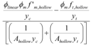
Compressive Strength
For a wall composed of hollow ungrouted blocks, or semi-solid ungrouted blocks, or solid blocks, the compressive strength values are readily obtained from CSA S304-14: Table 4. In MASS, when ignoring the effects of grout, the compressive strength value used is f’m,hollow . In MASS, when including the effects of grout for grouted walls, the compression strength of the masonry depends on the depth of the compression zone. If the depth of the compression zone falls in the face shell, the values for the hollow compressive strength,f’m,grouted can be used (CSA S304-14: Table 4). If the depth of the compression zone is greater than the width of the face shell, and the wall is fully grouted, the values for grouted compressive strength,f’m,hollow, can be used (CSA S304-14: Table 4). If the depth of the compression zone is greater than the width of the face shell, and the wall is partially grouted, an effective compressive strength,f’m,eff , is calculated. The weighted average compressive strength (effective compressive strength,f’m,eff ) is determined by averaging the compressive strengths of the grouted cells (f’m,grouted ) and the ungrouted cells (f’m,hollow) with respect to the relative areas:
 Where Agrouted is the grouted cross-sectional area of the wall, and Ahollow is the hollow cross-sectional area of the wall. The effective tensile strength can be calculated using the same principles.
![]() Note: This feature only affects the engineering calculations for partially grouted webs. For webs that are not grouted,
Note: This feature only affects the engineering calculations for partially grouted webs. For webs that are not grouted,
Agrouted=0 therefore
f’m,eff=f’m,hollow. For webs that are fully grouted,
Ahollow=0, therefore
f’m,eff = f’m’grouted .
Face Shell Thickness
The face shell thickness refers to the width of the face shell, or portion of a block between cell and outside surface of block side. Face shells are often tapered or flared as shown in Figure 4‑59: Face shell Profile‑, having varying thickness over the height of the block. The flare is introduced to facilitate picking up the block.
In general, face shell thickness depends on block size, with wider blocks having proportionately larger face shells.
Figure 4‑59: Face shell Profile
The effective face shell thickness, tf, of the block is the thickness to be used for design. It is the face shell thickness that develops from the placement of face shell mortar between the masonry units, and should not be confused with the actual minimum, average, or maximum thickness of the block shell.
The maximum face shell thickness is not displayed by the program, and cannot be altered by users. However, it is required by the program to determine the available space into which reinforcing steel bar can be placed. That is, the maximum face shell thickness is considered only indirectly; it is incorporated in the limits and tolerances on user input of steel bars in the cell cavities.
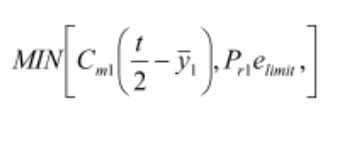
Eccentricity Limit
For unreinforced walls, the program verifies if the wall can be designed as a cracked section by determining the virtual eccentricity limit elimit=t/3 (CSA S304-14: 7.2.3) and comparing it to the actual virtual eccentricity e=Mf,Total/Pf . That is, if e<elimit the wall can be designed as a cracked section, if e≥elimit the wall must be designed as an uncracked section.
Moment
To view a full list of the moment design results:
- Click on the Detailed Results tab
- Click on the Moment tab
The Moment tab contains a table that provides detailed information about the axial and moment resistance of the wall. Since the program calculates the moment resistance of the wall ignoring and including the effects of the grout (if applicable), this tab shows all the variables and equations related to this process. Information about the reinforcement (number of bars per cell, bar spacing, reinforcement area, etc.) is also provided.
In general, the data presented in the Moment tab approximately corresponds to the calculations performed in the axial and moment and deflection design step.
The first set of variables displayed are the final, summarized axial and moment resistance calculations for the wall design. In the design shown in Figure 4‑60: Detailed Results (Moment), Mr=Mr1. This occurs if the compression zone falls within the face shell or because ignoring the effect of grout happens to provide the larger moment resistance. Further down, the axial and moment resistance calculations for when the effects of grout are ignored and included, are presented, as shown in Figure 4‑60: Detailed Results (Moment). As mentioned earlier, MASS employs a unique design approach; the program performs two moment capacity calculations: one that including the effect of grout and not including the effect grout (based on the philosophy that adding grout will not reduce the capacity of the walls).
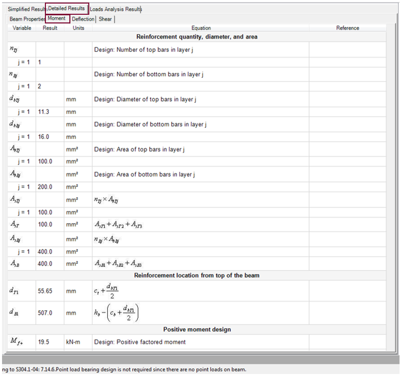
Figure 4‑60: Detailed Results (Moment)
Most variables displayed in the Detailed Results → Moment tab are variables commonly used and follow the convention presented in CSA S304-14. In cases where the variable/symbol is not governed by a specific equation, a description of the variable is provided instead. Variables and equations that require further explanation are discussed in the following subsections.
![]() Note: The two sets of axial resistance calculations (for when grout is ignored and included) are only provided if the wall design has grout. If the wall is not grouted, there is only one set of axial resistance calculations.
Note: The two sets of axial resistance calculations (for when grout is ignored and included) are only provided if the wall design has grout. If the wall is not grouted, there is only one set of axial resistance calculations.
In general, variables that contain a subscript ‘1’ are terms calculated ignoring the effects of grout (using f’m,hollow). Variables that contain a subscript ‘2’ are terms calculated including the effects of grout (using f’m,hollow if the compression zone depth fits within the first face shell, and using f’m’grouted if the compression zone depth exceeds the thickness of the first face shell).
Notice, however, that for reinforced walls, the label ‘1’ and ‘2’ may also be associated with the a particular steel layer (for instance Tx1, and Tx2).
Main Tension Steel (Reinforced Walls)
MASS allows users to place up to two reinforcing bars in a cell. The program selects the bar layer closest to the extreme tension fibre as the main tension steel layer. In the program, any information related to the main tension steel is always labelled with the subscript ‘1’ (that is:
Ts1, fs1, d1).
Figure 4‑61: Main Tension Steel and Figure 4‑62: Main Tension Steel (Top in Compression) illustrate how MASS selects the main tension steel.
|
Figure 4‑61: Main Tension Steel (Bottom in Compression) |
|
The main tension steel is the bar layer at the top when the bottom of the cross-section is in compression (Figure 4‑61: Main Tension Steel‑); and, the main tension steel is the bar layer at the bottom when the compression zone is at the top of the cross-section (Figure 4‑62: Main Tension Steel (Top in Compression)‑). MASS assumes the reinforcing steel is in compression as soon as the neutral axis depth reaches the main tension steel; that is, when c≥d1.
![]() Note: Vertical steel is not be taken into account for compression calculations in the design process; as it is extremely difficult to tie the bars together in a cell of a concrete block masonry wall. As a result, when the steel goes into compression it is assumed to carry zero force because it is untied and could buckle.
Note: Vertical steel is not be taken into account for compression calculations in the design process; as it is extremely difficult to tie the bars together in a cell of a concrete block masonry wall. As a result, when the steel goes into compression it is assumed to carry zero force because it is untied and could buckle.
Scrolling further down, the program provides the calculations used to account for slenderness effects. Slenderness effects are incorporated using the moment magnifier method. The variables follow the convention presented in CSA S304-14: 7.7.5, 7.7.6 (for unreinforced) and CSA S304-14: 10.7.3, 10.7.4 (for reinforced), thus no further explanation is required.
The program checks if the wall is slender (slenderness ratio greater than 30). If the wall is slender, special considerations are taken into account, as specified in CSA S304-14: 10.7.4.6 (pinned-pinned fixity conditions, reinforcement must yield, and wall must have a minimum thickness of 140 mm). The program also limits the amount of factored axial load applied to slender walls (CSA S304-14: 10.7.4.6.4).
![]() Note: Slender walls must be reinforced in accordance with CSA S304-14: 7.7.5.2.
Note: Slender walls must be reinforced in accordance with CSA S304-14: 7.7.5.2.
For unreinforced walls, the Detailed Results → Moment tab shows information about the uncracked and (or cracked) properties of the wall, as can be seen in Figure 4‑63: Detailed Results (Moment).
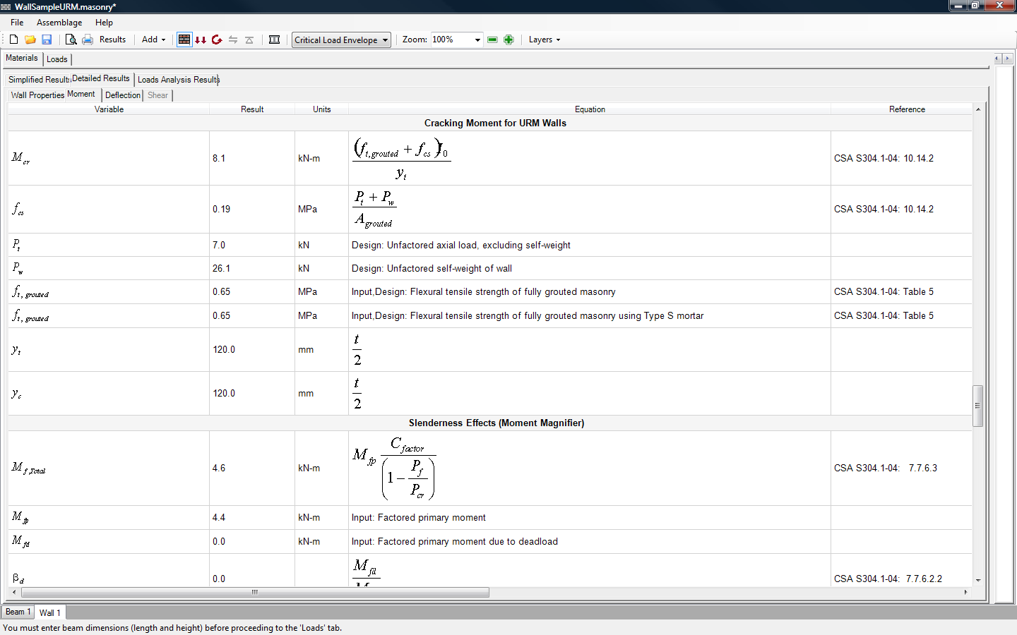
Figure 4‑63: Detailed Results (Moment)
Notice, that depending on if the wall is cracked, reinforced, and the eccentricity, a different moment equation may be used, as presented in Table 4‑6: Moment Resistance of Unreinforced Walls (Grout is Excluded or Ignored)‑. The simplified equations presented in Table 4‑6: Moment Resistance of Unreinforced Walls (Grout is Excluded or Ignored)‑ apply to unreinforced walls when grout is excluded, or ignored. Similar equations labelled with a subscript ‘2’ are used to describe the moment resistance when the effects of grout are included.
Table 4‑6: Moment Resistance of Unreinforced Walls (Grout is Excluded or Ignored)
|
Symbol |
Equation |
Description |
|
Mr1 |
MIN(Mr1+,Mr1-) |
A wall designed to remain uncracked carries a compressive masonry strength, as well as a tensile masonry strength (unlike cracked walls, where the tensile strength of masonry is neglected). The moment resistance of an uncracked section is determined by comparing the tensile and compressive strength of masonry. The smaller of these two values is taken as the moment resistance of the wall.
|
|
Mr1+ |
|
Factored moment resistance based on the compressive stress |
|
Mr1- |
|
Factored moment resistance based on the tensile stress. This equation can only be used if wall is designed to remain uncracked. |
|
Mequal1 |
|
This equation creates the cut-off point where the tensile strength of the wall can no longer be used. This occurs at the value Pequal1, when the compressive strength of the masonry and the tensile strength of the masonry are equal., that is, when Mr1+ = Mr1- |
|
Pequal1 |
|
This equation creates the cut-off point where the tensile strength of the wall can no longer be used. This occurs at the value Pequal1, when the compressive strength of the masonry and the tensile strength of the masonry are equal, that is, when Mr1+ = Mr1- |
|
Mr1 |
|
Factored moment resistance for a wall that can be designed as a cracked wall. |


Again, in the case of a grouted wall, the moment resistance of a cracked section is calculated for two instances: when the grout is included, and when it is not.
For more information on the design of out-of-plane walls, refer to the Wall Design Strategy section. For more information specifically relating to the equations used to determine the design of unreinforced wall and used to create the corresponding P-M Interaction diagram, refer to the P-M Interaction Diagram section.
Horizontal Out-of-Plane Bending
Notice that the equations presented thus far pertain to the vertical bending of the wall. Most walls are supported on three or four sides, and thus can experience both vertical bending and horizontal bending, as shown in Figure 4‑64: Vertical Flexure‑ and Figure 4‑65: Horizontal Flexure‑. It is not uncommon for a laterally loaded wall to experience flexure purely in the horizontal direction.
|
|
|
The approach to designing walls undergoing horizontal bending is similar to that of vertical bending. However, masonry assemblages are typically anisotropic, possessing a different capacity in horizontal direction than in the vertical direction. This is because in vertical flexure, bending stresses are parallel the head joints whereas for horizontal flexure, bending stresses are parallel to the bed joints. When approaching the ultimate load under horizontal bending, the head joints crack and no longer carry bending resistance. For further information on vertical bending, horizontal bending, and two-way bending please refer to page 316, 319, and 321 of [1], respectively.
 Warning: The current version of the Masonry Analysis Structural Systems software package designs for vertical flexure (vertical out-of-plane bending) only. MASS DOES NOT design walls to resist horizontal out-of-plane bending.
That being said, there is a guide available here which outlines a strategy for using MASS to analyze and design out-of-plane walls bending between horizontally spanning supports.
Deflection
To view a full list of the deflection design results:
- Click on the Detailed Results tab
- Click on the Deflection tab
The Deflection tab contains a table that provides detailed information about the wall service load deflection (including the effects of slenderness). The factors, variables, and equations used to determine the service load deflection, and the ones related to the secondary deflection (slenderness effects) are shown in Figure 4‑66: Detailed Results (Deflection).
In general, the data presented in this Deflection tab approximately corresponds to the calculations performed in the deflection design step.
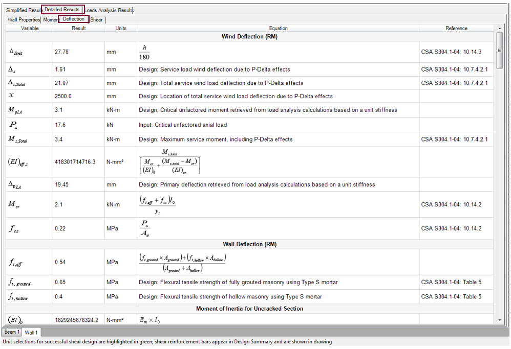
Figure 4‑66: Detailed Results (Deflection)
Most variables displayed in the Detailed Results → Deflection tab are variables commonly used and follow the convention presented in CSA S304-14. In cases where the variable/symbol is not governed by a specific equation, a description of the variable is provided instead. Variables and equations that may require further explanation are discussed in the following subsection.
Excluding Grout vs. Including Grout
Several variables under the ‘Moment of Inertia for Cracked Section (Excluding Grout)‘ and ‘Moment of Inertia for Cracked Section (Including Grout) ‘ headings shown in Figure 4‑67: Moment of Inertia for Cracked Section (Detailed Results) have the subscripts ‘no grout’ or ‘grout’. As stated previously, MASS employs a unique design approach; for fully or partially grouted walls, the program performs two calculations for the moment of inertia: one including the effect of grout and excluding the effect grout (based on the philosophy that adding grout should not reduce the capacity of the walls). For a wall that is partially or fully grouted, both calculations are provided, and the maximum of moment of inertia is selected.
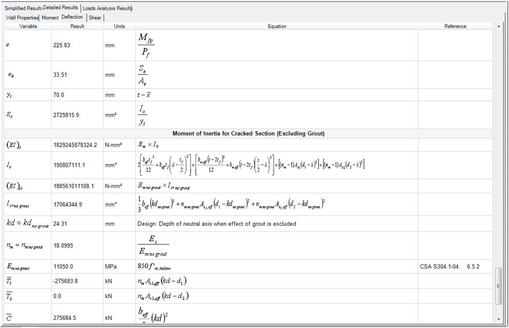
Figure 4‑67: Moment of Inertia for Cracked Section (Detailed Results)
![]() Note: MASS does not provide deflection calculations for unreinforced masonry walls. CSA S304 does not provide provisions for calculating the deflection of URM walls. The out-of-plane masonry walls do not deflect without significant cracking. For unreinforced masonry walls, the cracking permitted is heavily restricted. An unreinforced wall would typically fail in moment design anyway (before failing in deflection).
Note: MASS does not provide deflection calculations for unreinforced masonry walls. CSA S304 does not provide provisions for calculating the deflection of URM walls. The out-of-plane masonry walls do not deflect without significant cracking. For unreinforced masonry walls, the cracking permitted is heavily restricted. An unreinforced wall would typically fail in moment design anyway (before failing in deflection).
Shear
To view a full list of the shear design results:
- Click on the Detailed Results tab
- Click on the Shear tab
The Shear tab contains a table that provides detailed information about the shear design calculations, as shown in Figure 4‑68: Detailed Results (Shear). The program shows factors, variables, and equations for the shear and the sliding shear at the location of the critical section.
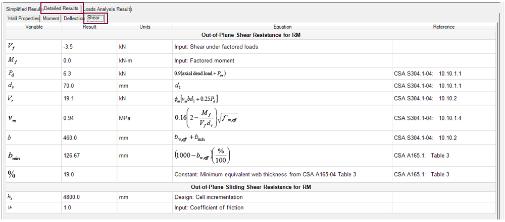
Figure 4‑68: Detailed Results (Shear)
In general, the data presented in this Shear tab approximately corresponds to the calculations performed in the shear design step. The variables displayed in the Detailed Results → Shear tab are variables commonly used and follow the convention presented in CSA S304-14. An exception may be the minimum web thickness,bmin.
Minimum Web Thickness
To calculate the out-of-plane shear resistance of walls, CSA S304-14: 10.10.3 indicates that the shear width b should include the width of unit webs and grouted cells. The web thickness varies bw,eff with the size of the masonry unit; CSA A165: Table 3 shows the minimum web thickness values for all sizes of standard concrete block units. The values of the equivalent web thickness as a percentage of the length of the unit are hard-coded into the program. The program uses these values to determine the minimum web thickness (bmin) of not grouted (hollow) or partially grouted masonry within the design length (1000 mm), that is
 The program sets the percentage value of the equivalent web thickness to 21 % for all concrete block sizes greater than 300 mm; and, it sets the percentage value of the equivalent web thickness to 15 % for all concrete block sizes lesser than 100 mm.
The shear width is then calculated by adding the width of grouted cells and the minimum web thickness within the design length b=bw,eff + bmin .
Continue Reading: Loads Analysis Results for Walls
Was this post helpful?