

P-M Interaction Diagram
Providing a deep dive into the specifics on how the Interaction Diagram is generated
Contents
After achieving a successful axial, moment and deflection design, the program creates an axial resistance Pr vs. moment resistance Mr diagram. The calculation procedure and the curves displayed in the P-M diagram depend on whether the wall is reinforced or not, and whether the masonry is hollow, partially grouted or fully grouted.
MASS also provides an envelope curve, based on the grout ignored and grout included curves drawn. The envelope curve indicates the bounds of acceptable Pr and Mr combinations, that is, those that cannot be exceeded by the combination of Pr and Mr that appears in the program.
P-M Interaction Diagram (Unreinforced Masonry)
The moment resistance Mr is determined and plotted for incremented values of the axial resistance Pr. The moment resistance calculations vary depending on whether the wall is designed as an uncracked or a cracked section.
The P-M interaction diagram for unreinforced masonry walls is created in three separate stages. The first stage, where the wall must remain uncracked (the curve is under the elimit line). The second stage or middle stage is governed by the elimit line, and how this line intersects with previous lines (design stages one and three). The third stage, where the wall can be designed as a cracked section (the curve is above the elimit line) and the moment resistance is calculated using the equivalent rectangular stress block. The following sections describe the methodology used for each situation.
Uncracked Moment Resistance (Tensile)
The uncracked tensile moment resistance line intersects with the elimit line, and the corresponding axial load resistance (Pgrey1(T) or Pgrey2(T) ) is less than the axial load resistance when the tensile moment resistance is equal to the compressive moment resistance (Pequal1 or Pequal2). See
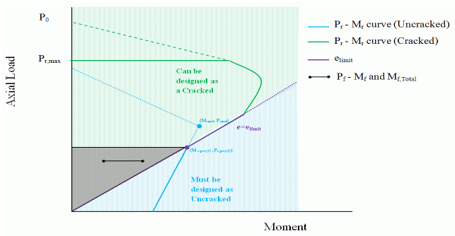
Figure 1: Uncracked Moment Resistance (Tensile)
Uncracked Moment Resistance (Compressive)
The elimit line intersects the compressive moment resistance line, and the corresponding axial load resistance (Pr,grey1(c)) or Pr,grey2(c)) is greater than the axial load resistance when the tensile moment resistance is equal to the compressive moment resistance (Pequal1 or Pequal2). See
Since, the program uses a safety factor ∅linear,to ensure that the uncracked moment resistance remains in a region that is governed by linear behaviour; the program plots the uncracked moment resistance up to where the tensile moment resistance is equal to the compressive moment resistance (Pequal1 or Pequal2). At this point, to avoid underestimating the capacity of the wall, a vertical line is drawn up to the elimit line, at the point
(Mr,grey1(c), Pr,grey1(c)) or Mr,grey2(c), Pr,grey 2(c)
.
Figure 2: Uncracked Moment Resistance (Compressive)
Cracked Moment Resistance (Tensile)
Cracked Moment Resistance (Compressive)
At the point where the moment resistance along the elimit line is no longer the smaller value (for the same axial resistance). The program continues calculating the moment resistance, Mr1 and, Mr2, of the cracked wall using the equivalent rectangular stress block, C1 , and, C2.
Grey zone
It is possible for the factored loads (Pf, Mf,Total) to fall inside the cracked portion of the P-M diagram, but at the same time have a corresponding uncracked moment resistance. To ensure that the program does not skip over a possible solution by assuming the design fails, when in fact the uncracked section provides enough resistance; the program uses the grey zone.
The grey zone is located above the elimit line, and extends up to the axial resistance where the elimit line intersects with the uncracked curve, Pgrey1 or Pgrey 2. Note that shaded grey zone is not displayed in the P-M diagram; it is shown in
When the factored loads fall within the grey zone, the program verifies both the uncracked and cracked moment resistance before establishing the success or failure of a design.
P-M Interaction Diagram (Reinforced Masonry)
MASS does not account for reinforcement in compression in the moment resistance calculations, since tying bars in walls is not easily accomplished. Consequently, in the case where compression zone depth is equal to the depth of the reinforcement, c=d1, where the steel transitions from being in tension (Mr,tension, Pr, tension) to being in compression (Mr,compression,Pr,compression), the moment resistance varies considerably upon the smallest increment of, c. This results in missing moment resistance and axial resistance data points in between this transition zone.
In order to create a smoother transition in the P-M diagram, while maintaining a conservative design, the program takes special design considerations depending on the case in which the transition zone is encountered.
Case 1
Case 1 occurs when the transition zone points (Mr,tension, Pr, tension) and (Mr,compression, Pr,compression) fall below the elimit line, and these point connect to form a line with a positive slope (
In order to obtain data points for the transition zone, the program divides the zone into two sections. First, a vertical line is drawn from (Mr,tension, Pr, tension) to the elimit line. And secondly, the elimit line is extended to(Mr,compression, Pr,compression), where the wall is treated as unreinforced.
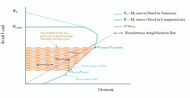
Figure 3: Transition Zone (Case 1)
Case 2a
Case 2a occurs when both transition points, (Mr,tension, Pr, tension) and
(Mr,compression, Pr,compression), fall above the elimit line (see
In order to obtain data points for the transition zone, the program draws a line connecting the points (Mr,tension, Pr, tension) and (Mr,compression, Pr,compression). Note, that this methodology is applied independent of whether the (Mr,compression, Pr,compression) is to the left or right of (Mr,tension, Pr, tension) , as long as both points are above the elimit line. The connecting line is governed by the following equation:

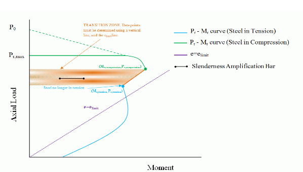
Figure 4: Transition Zone (Case 2a)
Case 2b
This case occurs when the steel in tension point (Mr,tension, Pr, tension) falls above the elimit line, and the steel in compression point (Mr,compression, Pr,compression) falls below the elimit line (see
For this particular case, since (Mr,compression, Pr,compression) falls below the elimit line, the program is concerned with the unreinforced wall cracking past the permitted limit (dictated by elimit). To account for this, the program determines the moment resistance from the linear equation used in Case 2a and compares it to the moment resistance along the elimit line, calculated as follows:
Mr=Prelimit
The smaller of the two moment values is used.
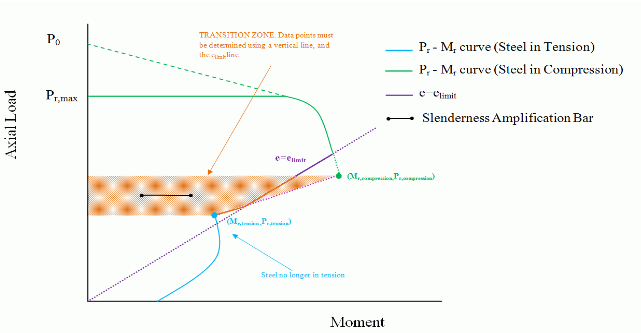 Figure 5: Transition Zone (Case 2b)
Case 3a
Case 3a occurs when steel in tension point (Mr,tension, Pr, tension) falls below the elimit line, and the steel in compression point (Mr,compression, Pr,compression) falls above the elimit line (see
In order to obtain data points for the transition zone, the program draws a line connecting the points (Mr,tension, Pr, tension) and (Mr,compression, Pr,compression). The connecting line is the same linear line provided in Case 2a.
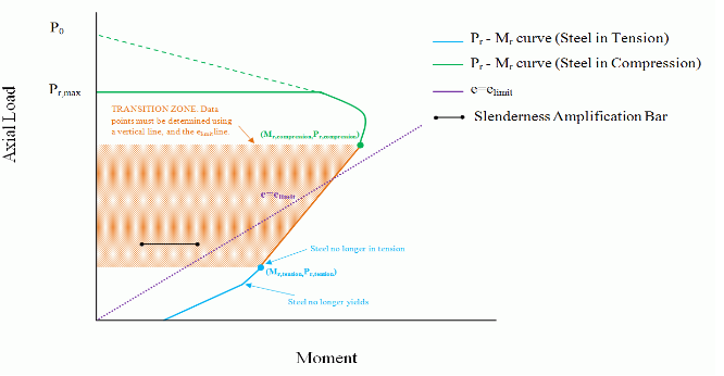
Figure 6: Transition Zone (Case 3a)
Case 3b
Case 3b occurs when both transition points, (Mr,tension, Pr, tension) and (Mr,compression,Pr,compression), fall below the elimit line (see
In order to obtain data points for the transition zone, the program draws a line connecting the points (Mr,tension, Pr, tension) and (Mr,compression, Pr,compression). The connecting line is governed by the equation shown in Case 2a.
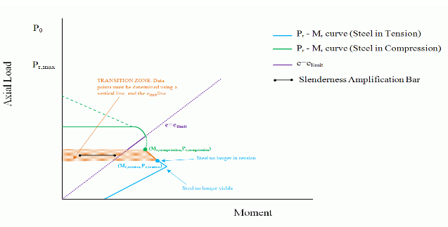
Figure 7: Transition Zone (Case 3b)
Continue Reading: P M Interaction Diagram Shear
Was this post helpful?